Statistical Analysis with R
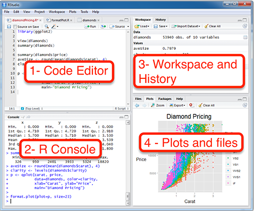
R Programming is more user-friendly for statistical analysis as you will see. The framework of RStudio consists of 4 sections:
Create a new R Script and import a package:
# This is how we import a package in R:
library(MASS)
If the package is not installed to your computer you can install it by typing:
install.packages('packagename')
However, throughout this course we are going to use only default libraries.
MASS package includes some datasets. You can see what kind of datasets the packages have from the 4. section of RStudio. Let’s take the Animals dataset:
data(Animals)
It takes some while to receive the data. Afterwards you can see the structure of the dataframe by:
View(Animals)
We have the animal names in the row indexes and two columns: Body weight and brain weight. It takes lot’s of efforts for doing a regression in Python as you would remember. However it is relatively easy in R:
lr = lm(brain ~ body, data = Animals)
summary(lr)
So we have the equation Summary is:
summary(lr)
Call:
lm(formula = brain ~ body, data = Animals)

Residuals:
   Min     1Q Median     3Q    Max
-576.0 -554.1 -438.1 -156.3 5138.5

Coefficients:
              Estimate Std. Error t value Pr(>|t|)
(Intercept)  5.764e+02  2.659e+02   2.168   0.0395 *
body        -4.326e-04  1.589e-02  -0.027   0.9785
---
Signif. codes:  0 ‘***’ 0.001 ‘**’ 0.01 ‘*’ 0.05 ‘.’ 0.1 ‘ ’ 1

Residual standard error: 1360 on 26 degrees of freedom
Multiple R-squared:  2.853e-05,	Adjusted R-squared:  -0.03843
F-statistic: 0.0007417 on 1 and 26 DF,  p-value: 0.9785
Let’s import another dataset:
data(Boston)
The description of the dataset:
crim
per capita crime rate by town.
zn
proportion of residential land zoned for lots over 25,000 sq.ft.
indus
proportion of non-retail business acres per town.
chas
Charles River dummy variable (= 1 if tract bounds river; 0 otherwise).
nox
nitrogen oxides concentration (parts per 10 million).
rm
average number of rooms per dwelling.
age
proportion of owner-occupied units built prior to 1940.
dis
weighted mean of distances to five Boston employment centres.
rad
index of accessibility to radial highways.
tax
full-value property-tax rate per \$10,000.
ptratio
pupil-teacher ratio by town.
black
1000(Bk - 0.63)^2 where Bk is the proportion of blacks by town.
lstat
lower status of the population (percent).
medv
median value of owner-occupied homes in \$1000s.
Let’s do OLS fit again:
> lr2 = lm(crim ~ ., data = Boston)
> summary(lr2)

Call:
lm(formula = crim ~ ., data = Boston)

Residuals:
   Min     1Q Median     3Q    Max
-9.924 -2.120 -0.353  1.019 75.051

Coefficients:
              Estimate Std. Error t value Pr(>|t|)
(Intercept)  17.033228   7.234903   2.354 0.018949 *
zn            0.044855   0.018734   2.394 0.017025 *
indus        -0.063855   0.083407  -0.766 0.444294
chas         -0.749134   1.180147  -0.635 0.525867
nox         -10.313535   5.275536  -1.955 0.051152 .
rm            0.430131   0.612830   0.702 0.483089
age           0.001452   0.017925   0.081 0.935488
dis          -0.987176   0.281817  -3.503 0.000502 ***
rad           0.588209   0.088049   6.680 6.46e-11 ***
tax          -0.003780   0.005156  -0.733 0.463793
ptratio      -0.271081   0.186450  -1.454 0.146611
black        -0.007538   0.003673  -2.052 0.040702 *
lstat         0.126211   0.075725   1.667 0.096208 .
medv         -0.198887   0.060516  -3.287 0.001087 **
---
Signif. codes:  0 ‘***’ 0.001 ‘**’ 0.01 ‘*’ 0.05 ‘.’ 0.1 ‘ ’ 1

Residual standard error: 6.439 on 492 degrees of freedom
Multiple R-squared:  0.454,	Adjusted R-squared:  0.4396
F-statistic: 31.47 on 13 and 492 DF,  p-value: < 2.2e-16
R is actually is programming language. In a way you can do everything you did in Python but in a different way. Each of them have their pros and cons (Python vs R).
One of the distinctive advantage of R is data visualization. Let’s import another dataset:
data("Rabbit")
View(Rabbit)
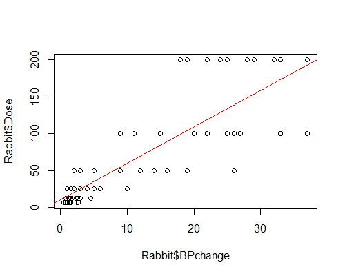
cor(Rabbit$BPchange, Rabbit$Dose)
cor() function gives the correlation between Dose and BPchange which is 0.831961. Let’s visualize this:
plot(Rabbit$BPchange, Rabbit$Dose)
abline(lm(Dose~BPchange, data = Rabbit), col = 'red')
abline() function draws the fit line of lm(Dose~BPchange, data = Rabbit) regression:
These datasets are ready-to-use datasets. So it is not too much trouble to make analysis or plot this data. Let’s import our latest movies dataset manipulated in the pandas lecture.
mv = read.csv('https://itueconomics.github.io/bil113e/assets/movies_new.csv')
We read the csv table and assigned it to the mv variable.
Unlike the Python, R has more built-in functions like plot, read.csv, lm, etc. All these functions are done with different library in Python. Let’s plot the number of movies in each categories:
barplot(colSums(mv[,5:23] == 'True'), las=2)
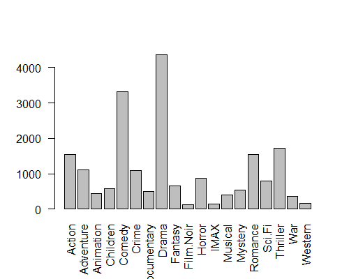
The tricky part is colSums(mv[,5:23] == 'True'). We had integration problem with the Python here. First we sliced the category columns of the data frame. Secondly True values are counted. The True values are not Boolean here. Because R has a syntax difference with Python in which all letters are capital for Boolean values like TRUE. So from R’s perspective they are string. We counted the True values and use colSums() functions to sum number of movies in each category. las attribute is for range of x and y labels. Try to change it and see what happens.
As you see most of the movies are Drama. So let’s fit a Logistic regression to find if a movie is Drama or not by controlling the other variables:
logitfit <- glm(Action ~ . , data = mv[,5:23], family = 'binomial')
Results:
summary(logitfit)
Call:
glm(formula = Action ~ ., family = "binomial", data = mv[, 5:23])

Deviance Residuals:
    Min       1Q   Median       3Q      Max
-2.3512  -0.4742  -0.3656  -0.1372   3.4350

Coefficients:
                Estimate Std. Error z value Pr(>|z|)
(Intercept)     -1.13060    0.08735 -12.943  < 2e-16 ***
AdventureTrue    1.67832    0.09216  18.211  < 2e-16 ***
AnimationTrue    0.08269    0.15831   0.522    0.601
ChildrenTrue    -1.62448    0.17633  -9.213  < 2e-16 ***
ComedyTrue      -0.99786    0.08840 -11.288  < 2e-16 ***
CrimeTrue        1.16635    0.09109  12.804  < 2e-16 ***
DocumentaryTrue -3.76842    0.51076  -7.378 1.61e-13 ***
DramaTrue       -1.43744    0.08264 -17.393  < 2e-16 ***
FantasyTrue      0.11149    0.12738   0.875    0.381
Film.NoirTrue   -2.32035    0.44261  -5.242 1.58e-07 ***
HorrorTrue      -1.19779    0.12350  -9.699  < 2e-16 ***
IMAXTrue         1.24013    0.22330   5.554 2.80e-08 ***
MusicalTrue     -2.16058    0.42166  -5.124 2.99e-07 ***
MysteryTrue     -0.96209    0.14832  -6.486 8.79e-11 ***
RomanceTrue     -0.90336    0.12419  -7.274 3.49e-13 ***
Sci.FiTrue       1.03569    0.09928  10.432  < 2e-16 ***
ThrillerTrue     0.79965    0.08337   9.591  < 2e-16 ***
WarTrue          1.41572    0.13706  10.329  < 2e-16 ***
WesternTrue      0.11889    0.20984   0.567    0.571
---
Signif. codes:  0 ‘***’ 0.001 ‘**’ 0.01 ‘*’ 0.05 ‘.’ 0.1 ‘ ’ 1

(Dispersion parameter for binomial family taken to be 1)

    Null deviance: 8288.9  on 9111  degrees of freedom
Residual deviance: 5920.2  on 9093  degrees of freedom
AIC: 5958.2

Number of Fisher Scoring iterations: 7
We can interpret those coefficients as positive, negative or neutral correlations with being a Drama movie. Now let’s measure how well our model makes predictions:
> sum(round(predict(logitfit, type = 'response')) == (mv$Action == 'True')) / length(mv$Action)
[1] 0.8651229
We have 86% accuracy, not bad! Let’s examine the structure of the code. predict(logitfit, type = 'response')) makes predictions using the model. But it gives us probability therefore we round the probabilities to 0 and 1. Afterwards we compare the true values using mv$Action == 'True'. This part gives the number of true matching. We divide it by total number of observations: length(mv$Action). It gives the accuracy of the econometric model.
Let’s do it for Titanic survival data:
titanic <- read.csv('https://itueconomics.github.io/bil113e/assets/titanic/train.csv')
logitfit2 <- glm(Survived ~ as.factor(Pclass)+
                   Sex + Age + SibSp + Parch + Fare +
                   is.na(Cabin) + Embarked,
                 data = titanic,
                 family = 'binomial')
summary(logitfit2)
Let’s score our model:
> sum(logitfit2$y == round(logitfit2$fitted.values)) / length(logitfit2$y)
[1] 0.8011204
We have very similar results with the sklearn. There is one major difference that data manipulation is done with less code in this case. You can compare them.